 WorkbookWorkbook
The Workbook shows results from calculations in tabular format.
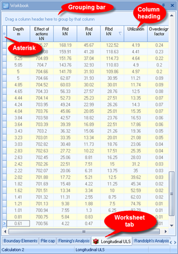
The data is presented on separate worksheets (e.g. Longitudanal ULS, Randolph’s Analysis etc.) which can be selected by clicking on the worksheet tabs at the bottom of the Workbook. Some worksheets have no data to display, in which case the worksheet displays a message to that effect.
In a worksheet, results are presented in a table where columns indicate properties and each row depicts a different result.
When the Workbook is visible, the Workbook tab is displayed on the Ribbon, which provides buttons relating to the panel.
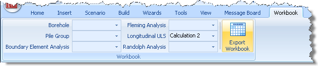
The Workbook tab indicates which worksheets have data to display and lets you switch between them.
It also enables you to Export the Workbook so that the results can be saved on an external program (e.g. Microsoft Excel) for future reference or printing.
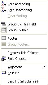
Right-click on a column heading for more options to sort and group the data as well as to remove that column.
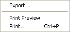
Right click elsewhere on the Workbook to reveal a second context menu allowing you to print or export the workbook.
The custom filter box allows you to select from a list of parameters to filter the data by.
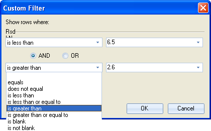
The list is accessible from drop down arrows in the left hand boxes.
Parameter values are entered in the right-hand boxes which have built-in calculators accessible from the drop down arrows.
Display a different selection of results
The default display only shows a small proportion of the available results.
Left-click on the Asterisk * in the top left corner of the table to see a drop-down list of all available columns
Left-click in the relevant tick boxes to show or hide the results you want displayed
 Or...
Or...
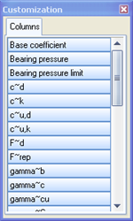
On the column context menu, choose Field Chooser to open a Customization dialog box
Left-click and drag columns onto the worksheet to add them to the results table
Left-click on a column heading and drag it across the worksheet to the desired position
Group identical values in a particular column
Drag the desired column into the Grouping bar found above the column headings or choose Group By This Field in the column context menu
This sorts all the results in ascending order by value for that column’s property. It also groups results with the same numerical value for that property
Left-clicking on the + button on each row expands the group to show all results with that value as well as the values of their other properties
Left-clicking on the drop down arrow in the column that has been dragged onto the Grouping bar allows you to filter the grouped results (see Filter results by their numerical values)
Sort the numerical values by a particular property
Left-click on the column heading that you want the data to be sorted by (data will ascend from lowest value) or select Sort Ascending on the column context menu
Left-click on the column heading again to reverse the order (data will descend from highest value) or select Sort Descending on the column context menu
By default, data is sorted in ascending order by value in the furthest left column.
Filter results by their numerical values
Left-click on the drop down arrow in the column heading of the property you want to filter by
Left-click to tick the boxes of the values that you want to keep
This hides all results apart from those which have one of the ticked numerical values for that property
Left-click on the drop down arrow and select (All) to restore filtered data
Left-click on the drop down arrow in the column heading of the property you want to filter by
Left-click on (Custom...) to open the custom filter box for more advanced filtering options
Current filters are displayed at the bottom of the workbook (above worksheet tabs).
Left-click on the checked tick box  to temporarily deselect the current filter
Left-click on the  button to cancel the current filter
To the right-hand side of the line describing the current filter, there is a drop down arrow which gives a list of previous filters so that they can be returned to easily. The Customize... button in the bottom right corner of the Workbook gives additional filter options.
To change the values shown in the results:
Left-click on the data cell you wish to change
Type a new value and press Enter
You can left-click on a data cell and drag the mouse down to select multiple data cells to change to the same value
Note: if data values are greyed out then they can’t be modified.
Right-click on a column to reveal its context menu and choose Best Fit to re-size the column. Choose Best Fit (all columns) to re-size all the columns
Right-click inside the panel to reveal the context menu and choose Export...
Select the folder you want to save the file in
Right-click inside the panel to reveal the context menu and choose Printor usethe keyboard shortcutCtrl+P